⏱️ Time Series Features

Time Series Features in KDP

Transform temporal data with powerful lag features, moving averages, differencing, rolling statistics, wavelet transforms, statistical features, and calendar features.

📋 Overview

Time series features enable processing of chronological data by creating transformations that capture temporal patterns and relationships. KDP provides specialized layers for common time series operations that maintain data ordering while enabling advanced machine learning on sequential data.

🚀 Types of Time Series Transformations

Transformation	Purpose	Example	When to Use
Lag Features	Create features from past values	Yesterday's sales, last week's sales	When past values help predict future ones
Rolling Statistics	Compute statistics over windows	7-day average, 30-day standard deviation	When trends or volatility matter
Differencing	Calculate changes between values	Day-over-day change in price	When changes are more important than absolute values
Moving Averages	Smooth data over time	7-day, 14-day, 28-day moving averages	When you need to reduce noise and focus on trends
Wavelet Transforms	Multi-resolution analysis of time series	Extracting coefficients at different scales	When you need to analyze signals at multiple scales or frequencies
Statistical Features	Extract comprehensive statistical features	Mean, variance, kurtosis, entropy, peaks	When you need a rich set of features summarizing time series properties
Calendar Features	Extract date and time components	Day of week, month, is_weekend, seasonality	When seasonal patterns related to calendar time are relevant

📝 Basic Usage

There are two ways to define time series features in KDP:

Option 1: Using Feature Type Directly

from kdp import PreprocessingModel, FeatureType

# Define features with simple types
features = {
    "sales": FeatureType.TIME_SERIES,  # Basic time series feature
    "date": FeatureType.DATE,          # Date feature for sorting
    "store_id": FeatureType.STRING_CATEGORICAL  # Grouping variable
}

# Create preprocessor
preprocessor = PreprocessingModel(
    path_data="sales_data.csv",
    features_specs=features
)

Option 2: Using TimeSeriesFeature Class (Recommended)

from kdp import PreprocessingModel, TimeSeriesFeature

# Create a time series feature for daily sales data
sales_ts = TimeSeriesFeature(
    name="sales",
    # Sort by date column to ensure chronological order
    sort_by="date",
    # Group by store to handle multiple time series
    group_by="store_id",
    # Create lag features for yesterday, last week, and two weeks ago
    lag_config={
        "lags": [1, 7, 14],
        "drop_na": True,
        "fill_value": 0.0,
        "keep_original": True
    }
)

# Define features using both approaches
features = {
    "sales": sales_ts,
    "date": "DATE",          # String shorthand for date feature
    "store_id": "STRING_CATEGORICAL"  # String shorthand for categorical
}

# Create preprocessor
preprocessor = PreprocessingModel(
    path_data="sales_data.csv",
    features_specs=features
)

🧠 Advanced Configuration

For comprehensive time series processing, configure multiple transformations in a single feature:

from kdp import TimeSeriesFeature, PreprocessingModel

# Complete time series configuration with multiple transformations
sales_feature = TimeSeriesFeature(
    name="sales",
    # Data ordering configuration
    sort_by="date",                    # Column to sort by
    sort_ascending=True,               # Sort chronologically
    group_by="store_id",               # Group by store

    # Lag feature configuration
    lag_config={
        "lags": [1, 7, 14, 28],        # Previous day, week, 2 weeks, 4 weeks
        "drop_na": True,               # Remove rows with insufficient history
        "fill_value": 0.0,             # Value for missing lags if drop_na=False
        "keep_original": True          # Include original values
    },

    # Rolling statistics configuration
    rolling_stats_config={
        "window_size": 7,              # 7-day rolling window
        "statistics": ["mean", "std", "min", "max"],  # Statistics to compute
        "window_stride": 1,            # Move window by 1 time step
        "drop_na": True                # Remove rows with insufficient history
    },

    # Differencing configuration
    differencing_config={
        "order": 1,                    # First-order differencing (t - (t-1))
        "drop_na": True,               # Remove rows with insufficient history
        "fill_value": 0.0,             # Value for missing diffs if drop_na=False
        "keep_original": True          # Include original values
    },

    # Moving average configuration
    moving_average_config={
        "periods": [7, 14, 28],        # Weekly, bi-weekly, monthly averages
        "drop_na": True,               # Remove rows with insufficient history
        "pad_value": 0.0               # Value for padding if drop_na=False
    },

    # Wavelet transform configuration
    wavelet_transform_config={
        "levels": 3,                   # Number of decomposition levels
        "window_sizes": [4, 8, 16],    # Optional custom window sizes for each level
        "keep_levels": "all",          # Which levels to keep (all or specific indices)
        "flatten_output": True,        # Whether to flatten multi-level output
        "drop_na": True                # Handle missing values
    },

    # TSFresh statistical features configuration
    tsfresh_feature_config={
        "features": ["mean", "std", "min", "max", "median"],  # Features to extract
        "window_size": None,           # Window size (None for entire series)
        "stride": 1,                   # Stride for sliding window
        "drop_na": True,               # Handle missing values
        "normalize": False             # Whether to normalize features
    },

    # Calendar feature configuration for date input
    calendar_feature_config={
        "features": ["month", "day", "day_of_week", "is_weekend"],  # Features to extract
        "cyclic_encoding": True,       # Use cyclic encoding for cyclical features
        "input_format": "%Y-%m-%d",    # Input date format
        "normalize": True              # Whether to normalize outputs
    }
)

# Create features dictionary
features = {
    "sales": sales_feature,
    "date": "DATE",
    "store_id": "STRING_CATEGORICAL"
}

# Create preprocessor with time series feature
preprocessor = PreprocessingModel(
    path_data="sales_data.csv",
    features_specs=features
)

⚙️ Key Configuration Parameters

Parameter	Description	Default	Notes
sort_by	Column used for ordering data	Required	Typically a date or timestamp column
sort_ascending	Sort direction	True	True for oldest→newest, False for newest→oldest
group_by	Column for grouping multiple series	None	Optional, for handling multiple related series
lags	Time steps to look back	None	List of integers, e.g. [1, 7] for yesterday and last week
window_size	Size of rolling window	7	Number of time steps to include in window
statistics	Rolling statistics to compute	["mean"]	Options: "mean", "std", "min", "max", "sum"
order	Differencing order	1	1=first difference, 2=second difference, etc.
periods	Moving average periods	None	List of integers, e.g. [7, 30] for weekly and monthly
levels	Number of wavelet decomposition levels	3	Higher values capture more scales of patterns
window_sizes	Custom window sizes for wavelet transform	None	Optional list of sizes, e.g. [4, 8, 16]
tsfresh_features	Statistical features to extract	["mean", "std", "min", "max", "median"]	List of statistical features to compute
calendar_features	Calendar components to extract	["month", "day", "day_of_week", "is_weekend"]	Date-based features extracted from timestamp
cyclic_encoding	Use sine/cosine encoding for cyclical features	True	Better captures cyclical nature of time features
drop_na	Remove rows with insufficient history	True	Set to False to keep all rows with padding

💡 Powerful Features

🔄 Automatic Data Ordering

KDP automatically handles the correct ordering of time series data:

from kdp import TimeSeriesFeature, PreprocessingModel

# Define a time series feature with automatic ordering
sales_ts = TimeSeriesFeature(
    name="sales",
    # Specify which column contains timestamps/dates
    sort_by="timestamp",
    # Sort in ascending order (oldest first)
    sort_ascending=True,
    # Group by store to create separate series per store
    group_by="store_id",
    # Simple lag configuration
    lag_config={"lags": [1, 7]}
)

# Create features dictionary
features = {
    "sales": sales_ts,
    "timestamp": "DATE",
    "store_id": "STRING_CATEGORICAL"
}

# Even with shuffled data, KDP will correctly order the features
preprocessor = PreprocessingModel(
    path_data="shuffled_sales_data.csv",
    features_specs=features
)

# The preprocessor handles ordering before applying transformations
model = preprocessor.build_preprocessor()

🌊 Wavelet Transform Analysis

Extract multi-resolution features from time series data:

from kdp import TimeSeriesFeature, PreprocessingModel

# Define a feature with wavelet transform
sensor_data = TimeSeriesFeature(
    name="sensor_readings",
    sort_by="timestamp",
    # Wavelet transform configuration
    wavelet_transform_config={
        "levels": 3,                # Number of decomposition levels
        "window_sizes": [4, 8, 16], # Increasing window sizes for multi-scale analysis
        "keep_levels": "all",       # Keep coefficients from all levels
        "flatten_output": True      # Flatten coefficients into feature vector
    }
)

# Create features dictionary
features = {
    "sensor_readings": sensor_data,
    "timestamp": "DATE"
}

# Create preprocessor for signal analysis
preprocessor = PreprocessingModel(
    path_data="sensor_data.csv",
    features_specs=features
)

# The wavelet transform decomposes the signal into different frequency bands,
# helping to identify patterns at multiple scales

📊 Statistical Feature Extraction

Automatically extract rich statistical features from time series:

from kdp import TimeSeriesFeature, PreprocessingModel

# Define a feature with statistical features extraction
ecg_data = TimeSeriesFeature(
    name="ecg_signal",
    sort_by="timestamp",
    # Statistical feature extraction
    tsfresh_feature_config={
        "features": [
            "mean", "std", "min", "max", "median",
            "abs_energy", "count_above_mean", "count_below_mean",
            "kurtosis", "skewness"
        ],
        "window_size": 100,  # Extract features from windows of 100 points
        "stride": 50,        # Slide window by 50 points
        "normalize": True    # Normalize extracted features
    }
)

# Create features dictionary
features = {
    "ecg_signal": ecg_data,
    "timestamp": "DATE",
    "patient_id": "STRING_CATEGORICAL"
}

# Create preprocessor
preprocessor = PreprocessingModel(
    path_data="ecg_data.csv",
    features_specs=features
)

# The statistical features capture important characteristics of the signal
# without requiring domain expertise to manually design features

📅 Calendar Feature Integration

Extract and encode calendar features directly from date inputs:

from kdp import TimeSeriesFeature, PreprocessingModel

# Define a feature with calendar feature extraction
traffic_data = TimeSeriesFeature(
    name="traffic_volume",
    sort_by="timestamp",
    group_by="location_id",

    # Lag features for short-term patterns
    lag_config={"lags": [1, 2, 3, 24, 24*7]},  # Hours back

    # Calendar features for temporal patterns
    calendar_feature_config={
        "features": [
            "month", "day_of_week", "hour", "is_weekend",
            "is_month_start", "is_month_end"
        ],
        "cyclic_encoding": True,     # Use sine/cosine encoding for cyclical features
        "input_format": "%Y-%m-%d %H:%M:%S"  # Datetime format
    }
)

# Create features dictionary
features = {
    "traffic_volume": traffic_data,
    "timestamp": "DATE",
    "location_id": "STRING_CATEGORICAL"
}

# Create preprocessor for traffic prediction
preprocessor = PreprocessingModel(
    path_data="traffic_data.csv",
    features_specs=features
)

# Calendar features automatically capture important temporal patterns
# like rush hour traffic, weekend effects, and monthly patterns

🔧 Real-World Examples

📈 Retail Sales Forecasting

from kdp import PreprocessingModel, TimeSeriesFeature, DateFeature, CategoricalFeature

# Define features for sales forecasting
features = {
    # Time series features for sales data
    "sales": TimeSeriesFeature(
        name="sales",
        sort_by="date",
        group_by="store_id",
        # Recent sales and same period in previous years
        lag_config={
            "lags": [1, 2, 3, 7, 14, 28, 365, 365+7],
            "keep_original": True
        },
        # Weekly and monthly trends
        rolling_stats_config={
            "window_size": 7,
            "statistics": ["mean", "std", "min", "max"]
        },
        # Day-over-day changes
        differencing_config={
            "order": 1,
            "keep_original": True
        },
        # Weekly, monthly, quarterly smoothing
        moving_average_config={
            "periods": [7, 30, 90]
        },
        # Calendar features for seasonal patterns
        calendar_feature_config={
            "features": ["month", "day_of_week", "is_weekend", "is_holiday"],
            "cyclic_encoding": True
        }
    ),

    # Store features
    "store_id": CategoricalFeature(
        name="store_id",
        embedding_dim=8
    ),

    # Product category
    "product_category": CategoricalFeature(
        name="product_category",
        embedding_dim=8
    )
}

# Create preprocessor
sales_forecaster = PreprocessingModel(
    path_data="sales_data.csv",
    features_specs=features,
    output_mode="concat"
)

# Build preprocessor
result = sales_forecaster.build_preprocessor()

📊 Stock Price Analysis with Advanced Features

from kdp import PreprocessingModel, TimeSeriesFeature, NumericalFeature, CategoricalFeature

# Define features for financial analysis
features = {
    # Price as time series
    "price": TimeSeriesFeature(
        name="price",
        sort_by="date",
        group_by="ticker",
        # Recent prices and historical patterns
        lag_config={
            "lags": [1, 2, 3, 5, 10, 20, 60],  # Days back
            "keep_original": True
        },
        # Trend analysis
        rolling_stats_config={
            "window_size": 20,  # Trading month
            "statistics": ["mean", "std", "min", "max"]
        },
        # Multi-scale price patterns with wavelet transform
        wavelet_transform_config={
            "levels": 3,  # Capture short, medium, and long-term patterns
            "flatten_output": True
        },
        # Statistical features for price characteristics
        tsfresh_feature_config={
            "features": ["mean", "variance", "skewness", "kurtosis",
                         "abs_energy", "count_above_mean", "longest_strike_above_mean"]
        }
    ),

    # Volume information
    "volume": TimeSeriesFeature(
        name="volume",
        sort_by="date",
        group_by="ticker",
        lag_config={"lags": [1, 5, 20]},
        rolling_stats_config={
            "window_size": 20,
            "statistics": ["mean", "std"]
        }
    ),

    # Market cap
    "market_cap": NumericalFeature(name="market_cap"),

    # Sector/industry
    "sector": CategoricalFeature(
        name="sector",
        embedding_dim=12
    ),

    # Date feature with calendar effects
    "date": TimeSeriesFeature(
        name="date",
        calendar_feature_config={
            "features": ["month", "day_of_week", "is_month_start", "is_month_end", "quarter"],
            "cyclic_encoding": True
        }
    )
}

# Create preprocessor for stock price prediction
stock_predictor = PreprocessingModel(
    path_data="stock_data.csv",
    features_specs=features,
    output_mode="concat"
)

⚕️ Patient Monitoring with Advanced Features

from kdp import PreprocessingModel, TimeSeriesFeature, NumericalFeature, CategoricalFeature

# Define features for patient monitoring
features = {
    # Vital signs as time series
    "heart_rate": TimeSeriesFeature(
        name="heart_rate",
        sort_by="timestamp",
        group_by="patient_id",
        # Recent measurements
        lag_config={
            "lags": [1, 2, 3, 6, 12, 24],  # Hours back
            "keep_original": True
        },
        # Short and long-term trends
        rolling_stats_config={
            "window_size": 6,  # 6-hour window
            "statistics": ["mean", "std", "min", "max"]
        },
        # Extract rich statistical features automatically
        tsfresh_feature_config={
            "features": ["mean", "variance", "abs_energy", "count_above_mean",
                        "skewness", "kurtosis", "maximum", "minimum"],
            "window_size": 24  # 24-hour window for comprehensive analysis
        },
        # Multi-scale analysis for pattern detection
        wavelet_transform_config={
            "levels": 2,
            "flatten_output": True
        }
    ),

    # Blood pressure
    "blood_pressure": TimeSeriesFeature(
        name="blood_pressure",
        sort_by="timestamp",
        group_by="patient_id",
        lag_config={
            "lags": [1, 6, 12, 24]
        },
        rolling_stats_config={
            "window_size": 12,  # 12-hour window
            "statistics": ["mean", "std"]
        },
        # Extract statistical patterns
        tsfresh_feature_config={
            "features": ["mean", "variance", "maximum", "minimum"]
        }
    ),

    # Body temperature
    "temperature": TimeSeriesFeature(
        name="temperature",
        sort_by="timestamp",
        group_by="patient_id",
        lag_config={
            "lags": [1, 2, 6, 12]
        },
        rolling_stats_config={
            "window_size": 6,
            "statistics": ["mean", "min", "max"]
        }
    ),

    # Patient demographics
    "age": NumericalFeature(name="age"),
    "gender": CategoricalFeature(name="gender"),
    "diagnosis": CategoricalFeature(
        name="diagnosis",
        embedding_dim=16
    ),

    # Time information with calendar features
    "timestamp": TimeSeriesFeature(
        name="timestamp",
        calendar_feature_config={
            "features": ["hour", "day_of_week", "is_weekend", "month"],
            "cyclic_encoding": True,
            "normalize": True
        }
    )
}

# Create preprocessor for patient risk prediction
patient_monitor = PreprocessingModel(
    path_data="patient_data.csv",
    features_specs=features,
    output_mode="concat"
)

# The combination of lag features, statistical features, and wavelet transform
# enables detection of complex patterns in vital signs, while calendar features
# capture temporal variations in patient condition by time of day and day of week

💎 Pro Tips

🔍 Choose Meaningful Lag Features

When selecting lag indices, consider domain knowledge about your data:

• For daily data: include 1 (yesterday), 7 (last week), and 30 (last month)
• For hourly data: include 1, 24 (same hour yesterday), 168 (same hour last week)
• For seasonal patterns: include 365 (same day last year) for annual data
• For quarterly financials: include 1, 4 (same quarter last year)

This captures daily, weekly, and seasonal patterns that might exist in your data.

📊 Combine Multiple Transformations

Different time series transformations capture different aspects of your data:

• Lag features: Capture direct dependencies on past values
• Rolling statistics: Capture trends and volatility
• Differencing: Captures changes and removes trend
• Moving averages: Smooths noise and highlights trends

Using these together creates a rich feature set that captures various temporal patterns.

⚠️ Handle the Cold Start Problem

New time series may not have enough history for lag features:

# Gracefully handle new entities with insufficient history
sales_ts = TimeSeriesFeature(
    name="sales",
    sort_by="date",
    group_by="store_id",
    lag_config={
        "lags": [1, 7],
        "drop_na": False,     # Keep rows with missing lags
        "fill_value": 0.0     # Use 0 for missing values
    }
)

# Alternative approach for handling new stores
features = {
    "sales": sales_ts,
    "store_age": NumericalFeature(name="store_age"),  # Track how long the store has existed
    "date": "DATE",
    "store_id": "STRING_CATEGORICAL"
}

🔬 Advanced Time Series Feature Engineering

The new advanced time series features provide powerful tools for extracting patterns:

• Wavelet Transforms: Ideal for capturing multi-scale patterns and transient events. Use higher levels (3-5) for more decomposition detail.
• Statistical Features: The TSFresh-inspired features automatically extract a comprehensive set of statistical descriptors that would be time-consuming to calculate manually.
• Calendar Features: Combine with cyclic encoding to properly represent the circular nature of time (e.g., December is close to January).

For optimal results, combine these advanced features with traditional ones:

# Comprehensive time series feature engineering
sensor_feature = TimeSeriesFeature(
    name="sensor_data",
    sort_by="timestamp",

    # Traditional features
    lag_config={"lags": [1, 2, 3]},
    rolling_stats_config={"window_size": 10, "statistics": ["mean", "std"]},

    # Advanced features
    wavelet_transform_config={"levels": 3},
    tsfresh_feature_config={"features": ["mean", "variance", "abs_energy"]},
    calendar_feature_config={"features": ["hour", "day_of_week"]}
)

# This combination captures temporal dependencies (lags),
# local statistics (rolling stats), multi-scale patterns (wavelets),
# global statistics (tsfresh), and temporal context (calendar)

📊 Model Architecture Diagrams

Basic Time Series Feature

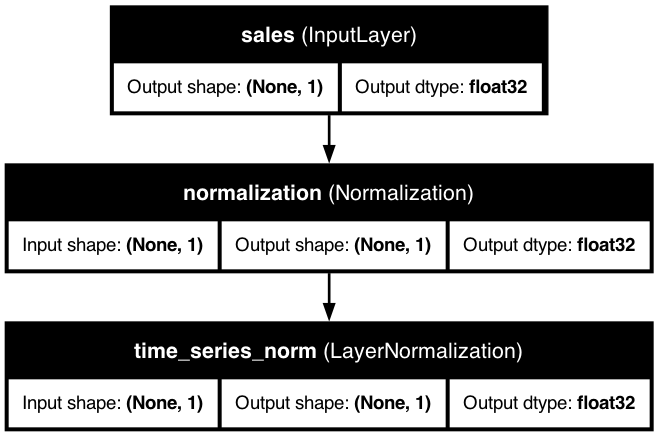
A basic time series feature with date sorting and group handling, showing how KDP integrates time series data with date features and categorical grouping variables.

Time Series with Lag Features

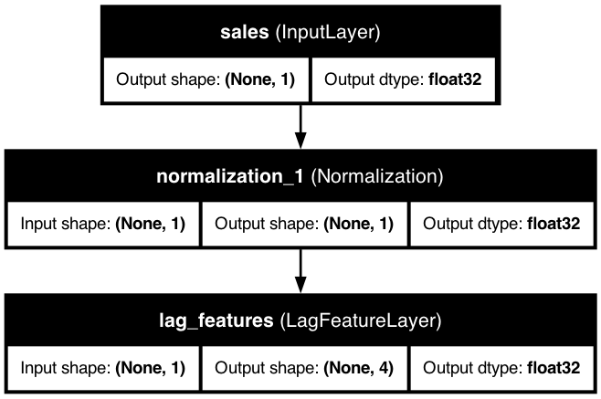
This diagram shows how lag features are integrated into the preprocessing model, allowing the model to access historical values from previous time steps.

Time Series with Moving Averages

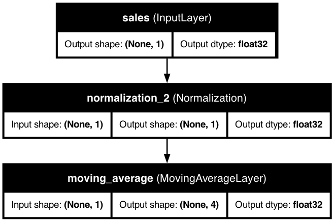
Moving averages smooth out noise in the time series data, highlighting underlying trends. This diagram shows how KDP implements moving average calculations in the preprocessing pipeline.

Time Series with Differencing

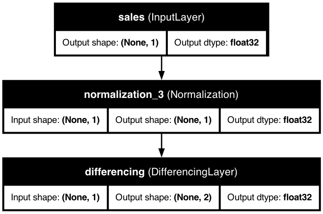
Differencing captures changes between consecutive time steps, helping to make time series stationary. This diagram shows the implementation of differencing in the KDP architecture.

Time Series with All Features

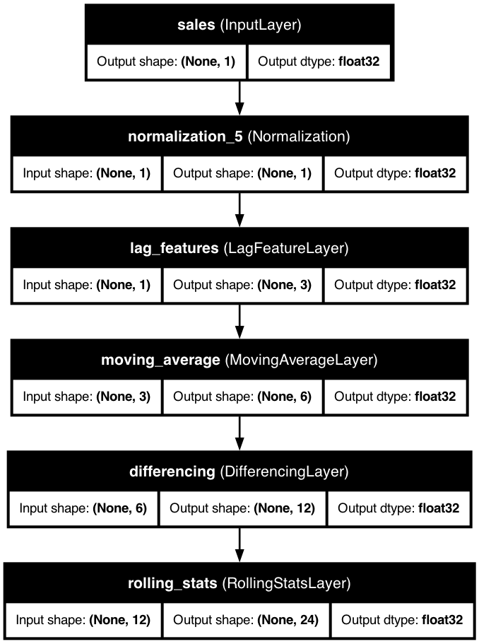
A comprehensive time series preprocessing pipeline that combines lag features, rolling statistics, differencing, and moving averages to capture all aspects of the temporal patterns in the data.

🔗 Related Topics

🏷️ Categorical Features 🔢 Numerical Features 🧩 Custom Preprocessing Layers 📈 Time Series Forecasting Examples

---

← Text Features Image Features →

🔍 Inference with Time Series Features

Time series preprocessing requires special consideration during inference. Unlike static features, time series transformations depend on historical data and context.

Minimal Requirements for Inference

Transformation	Minimum Data Required	Notes
Lag Features	max(lags) previous time points	If largest lag is 14, you need 14 previous data points
Rolling Statistics	window_size previous points	For a 7-day window, you need 7 previous points
Differencing	order previous points	First-order differencing requires 1 previous point
Moving Averages	max(periods) previous points	For periods [7,14,28], you need 28 previous points
Wavelet Transform	2^levels previous points	For 3 levels, you need at least 8 previous points

Example: Single-Point Inference

For single-point or incremental inference with time series features:

# INCORRECT - Will fail with time series features
single_point = {"date": "2023-06-01", "store_id": "Store_1", "sales": 150.0}
prediction = model.predict(single_point)  # ❌ Missing historical context

# CORRECT - Include historical context
inference_data = {
    "date": ["2023-05-25", "2023-05-26", ..., "2023-06-01"],  # Include history
    "store_id": ["Store_1", "Store_1", ..., "Store_1"],       # Same group
    "sales": [125.0, 130.0, ..., 150.0]                       # Historical values
}
prediction = model.predict(inference_data)  # ✅ Last row will have prediction

Strategies for Ongoing Predictions

For forecasting multiple steps into the future:

# Multi-step forecasting with KDP
import pandas as pd

# 1. Start with historical data
history_df = pd.DataFrame({
    "date": pd.date_range("2023-01-01", "2023-05-31"),
    "store_id": "Store_1",
    "sales": historical_values  # Your historical data
})

# 2. Create future dates to predict
future_dates = pd.date_range("2023-06-01", "2023-06-30")
forecast_horizon = len(future_dates)

# 3. Initialize with history
working_df = history_df.copy()

# 4. Iterative forecasting
for i in range(forecast_horizon):
    # Prepare next date to forecast
    next_date = future_dates[i]
    next_row = pd.DataFrame({
        "date": [next_date],
        "store_id": ["Store_1"],
        "sales": [None]  # Unknown value we want to predict
    })

    # Add to working data
    temp_df = pd.concat([working_df, next_row])

    # Make prediction (returns all rows, take last one)
    prediction = model.predict(temp_df).iloc[-1]["sales"]

    # Update the working dataframe with the prediction
    next_row["sales"] = prediction
    working_df = pd.concat([working_df, next_row])

# Final forecast is in the last forecast_horizon rows
forecast = working_df.tail(forecast_horizon)

Key Considerations for Inference

• Group Integrity: Maintain the same groups used during training
• Chronological Order: Ensure data is properly sorted by time
• Sufficient History: Provide enough history for each group
• Empty Fields: For auto-regressive forecasting, leave future values as None or NaN
• Overlapping Windows: For multi-step forecasts, consider whether predictions should feed back as inputs